Sabattier
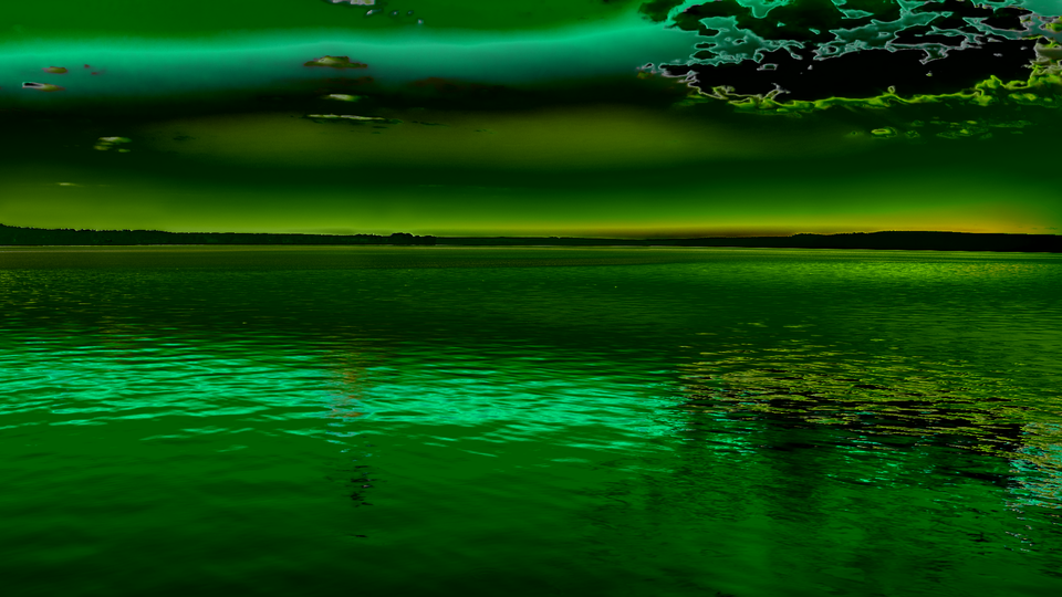
 Sabattier applying pseudo-solarization with Mackie line edge glow to create surreal, partially tone-reversed imagery.
Overview
Sabattier recreates the photographic darkroom technique of pseudo-solarization, where a partially developed print is briefly re-exposed to light. Midtone regions undergo partial tonal reversal while shadows and highlights remain relatively stable, producing a surreal, metallic appearance. The program computes this effect in real time by measuring each pixel's distance from the midtone center and subtracting a proportional dip, creating the characteristic tonal fold that defines the Sabattier effect.
The defining artifact of darkroom solarization: the Mackie line: is reproduced. In the darkroom, bromide ions released during development migrate laterally and inhibit development at tonal boundaries, leaving bright luminous borders where light and dark regions meet. Sabattier generates this artifact digitally via horizontal gradient detection: wherever the solarized luminance changes sharply from pixel to pixel, an additive glow appears along the boundary.
Beyond straight recreation, Sabattier offers creative extensions that go well beyond what a darkroom could achieve. Independent per-channel solarization, selectable curve shapes, equidensity contour mode, and metallic tinting expand the palette from subtle vintage warmth to aggressive digital abstraction.
Sabattier uses zero block RAM: the solarization curve is computed piecewise, not stored in a lookup table.
What's In a Name?
The effect is named after Armand Sabatier, the French scientist who first documented the phenomenon of tonal reversal through re-exposure in 1862. (The double-t spelling Sabattier entered popular use through a historical transcription error and became the accepted name for the effect.) The term pseudo-solarization distinguishes this darkroom accident from true solarization (caused by extreme overexposure of the negative itself). Man Ray famously popularized the technique in the 1930s, using it to create otherworldly portraits with glowing contour lines (the Mackie lines that Sabattier reproduces.)
Quick Start
- Turn Y Inversion (Knob 1) clockwise to about 75%. The midtones fold: areas near middle gray darken while highlights and shadows remain anchored. This is the core Sabattier effect.
- Increase Mackie Gain (Knob 3) to about 50%. Bright edge lines appear at tonal boundaries: the Mackie lines. Adjust Threshold (Knob 6) to control how much gradient is needed to trigger them.
- Turn Mackie Width (Knob 4) clockwise. The sharp edge lines soften and bloom outward, creating a glowing halo along each boundary.
- Toggle Curve Shape (Switch 10) from S-Curve to W-Curve. The single midtone dip splits into two, creating additional tonal folds at the quarter tones.
Parameters
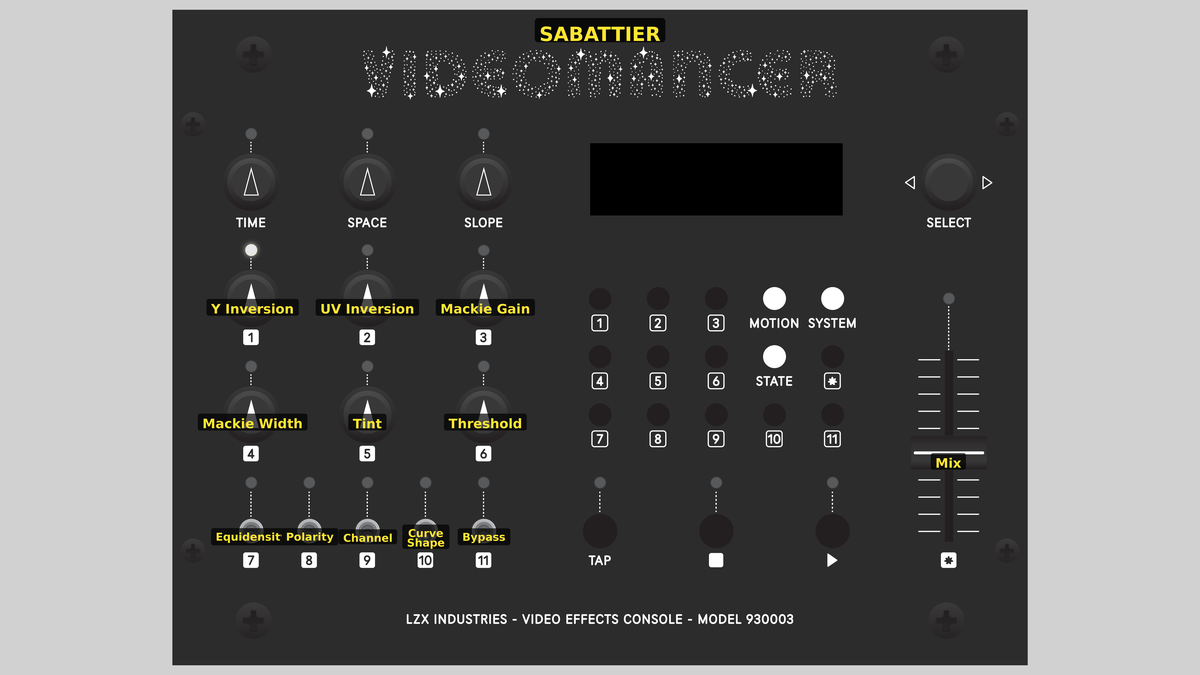 Videomancer's front panel with Sabattier active. Knobs 1–6 (top two rows of left cluster), Toggle switches 7–11 (bottom row of left cluster), Fader 12 (right side).
Knob 1 — Y Inversion
| Property | Value |
|---|---|
| Range | 0.0% – 100.0% |
| Default | 50.0% |
Y Inversion controls the depth of solarization applied to the luminance channel. At 0%, fully counterclockwise, no tonal reversal occurs: the luminance passes through unchanged. As the value increases, midtones are progressively folded downward: pixels near mid-gray darken while shadows and highlights remain stable. At 100%, the dip reaches its maximum depth. The effect is strongest at the midtone center (512 in S-curve mode) and tapers off toward the extremes, creating the signature triangular tonal fold of pseudo-solarization.
Start with Y Inversion around 50% to see the effect clearly without losing too much midtone detail. Higher values create increasingly dramatic tonal reversal.
Knob 2 — UV Inversion
| Property | Value |
|---|---|
| Range | 0.0% – 100.0% |
| Default | 0.0% |
UV Inversion controls the depth of solarization applied to the chrominance channels. This parameter is only active when Channel (Switch 9) is set to YUV. At 0%, chroma passes through unchanged. As the value increases, color values near the midpoint of each chroma axis are folded downward, creating surreal color shifts where saturated midtones desaturate or flip. At 100%, the chroma dip is at maximum depth.
Knob 3 — Mackie Gain
| Property | Value |
|---|---|
| Range | 0.0% – 100.0% |
| Default | 50.0% |
Mackie Gain controls the brightness of the Mackie line edge glow. At 0%, no edge glow is applied: even where tonal boundaries exist, no bright contour line appears. Increasing the value amplifies the detected gradient into a visible additive overlay. At 100%, the Mackie lines are at their brightest, tracing luminous borders along every significant tonal boundary in the solarized image. The glow is clamped to prevent overflow.
Knob 4 — Mackie Width
| Property | Value |
|---|---|
| Range | 0.0% – 100.0% |
| Default | 0.0% |
Mackie Width controls how far the edge glow spreads beyond the detected boundary. At 0%, the Mackie lines are sharp, single-pixel edges. As the value increases, an IIR (infinite impulse response) lowpass filter blends each new edge sample with the previous output, causing the glow to smear horizontally and bloom outward. At 100%, the glow spreads broadly, creating a soft halo around every tonal boundary.
The IIR filter operates horizontally along each scan line. Mackie Width does not affect the vertical extent of the glow (that is determined solely by the source imagery.)
Knob 5 — Tint
| Property | Value |
|---|---|
| Range | 0.0% – 100.0% |
| Default | 0.0% |
Tint applies a metallic color shift to the processed image. The tint amount is modulated by luminance: brighter areas receive more tinting. At 0%, no tint is applied. As the value increases, the U channel is shifted upward and the V channel is shifted downward by a luminance-proportional amount, creating a cool blue-cyan cast in bright regions. At 100%, the color shift is at its maximum.
Knob 6 — Threshold
| Property | Value |
|---|---|
| Range | 0.0% – 100.0% |
| Default | 0.0% |
Threshold sets the minimum gradient strength required for Mackie lines to appear. At 0%, even the smallest tonal transition triggers an edge glow. As the value increases, only sharper, more prominent boundaries produce Mackie lines: subtle gradients are gated off. At 100%, only the most extreme tonal edges survive. Use Threshold to clean up noisy or busy images where too many Mackie lines clutter the result.
Threshold and Mackie Gain work together. A higher Threshold suppresses weak edges while Gain amplifies the survivors. Use them in tandem to isolate just the strongest contour lines.
Switch 7 — Equidensity
| Property | Value |
|---|---|
| Off | Off |
| On | On |
| Default | Off |
Equidensity switches between normal solarization and equidensity contour mode. With the switch set to Off, the standard solarization dip is applied. With the switch set to On, the dip is doubled and clamped, creating sharp contour bands where the proximity function peaks: the image is divided into luminance zones separated by dark boundary lines. This is the digital equivalent of equidensity film, a specialist material used in scientific imaging to visualize iso-luminance contours.
Switch 8 — Polarity
| Property | Value |
|---|---|
| Off | Positive |
| On | Negative |
| Default | Positive |
Polarity inverts the input luminance before all processing. With the switch set to Positive, the original luminance is used. With the switch set to Negative, the luminance is complemented (1023 − Y) at the very first pipeline stage, reversing which tones are treated as shadows and which as highlights. Because the solarization curve is symmetric around its peak, inverting polarity shifts the dip along the tonal axis, changing which regions fold.
Switch 9 — Channel
| Property | Value |
|---|---|
| Off | Y Only |
| On | YUV |
| Default | Y Only |
Channel selects whether solarization affects only luminance or all three channels. With the switch set to Y Only, the UV Inversion control has no effect and chrominance passes through unchanged. With the switch set to YUV, the UV channels also undergo proximity-based tonal folding controlled by UV Inversion (Knob 2). YUV mode produces more dramatic color shifts, especially in saturated source material.
Switch 10 — Curve Shape
| Property | Value |
|---|---|
| Off | S-Curve |
| On | W-Curve |
| Default | S-Curve |
Curve Shape selects the proximity function used for solarization. With the switch set to S-Curve, a single triangle function peaks at the midpoint (value 512), creating one tonal fold. With the switch set to W-Curve, two triangle peaks appear at the quarter points (values 256 and 768), creating two tonal folds that divide the image into more complex tonal zones. The W-Curve produces additional contour lines and a more intricate solarization pattern.
Switch 11 — Metallic
| Property | Value |
|---|---|
| Off | Off |
| On | On |
| Default | Off |
Metallic forces the tint amount to its maximum value regardless of the Tint knob position. With the switch set to Off, the Tint knob controls the tint amount normally. With the switch set to On, the tint system operates at full strength, producing a strong blue-cyan metallic sheen in bright areas. This is a shortcut to the most extreme metallic appearance without needing to find the knob position.
Fader 12 — Mix
| Property | Value |
|---|---|
| Range | 0.0% – 100.0% |
| Default | 100.0% |
Mix crossfades between the dry (unprocessed) and wet (solarized) signal. At 0%, fully left, the output is the original input: no solarization is visible. At 100%, fully right, the output is entirely the processed signal. Intermediate values blend the two, allowing subtle integration of the Sabattier effect into the source image.
Background
Solarization in the darkroom
True solarization occurs when photographic film receives so much light that the silver halide crystals begin to reverse their response: shadows become highlights and vice versa. Pseudo-solarization, the Sabattier effect, is a related but distinct phenomenon. A partially developed print is briefly exposed to white light during development; the undeveloped silver halide in the lighter areas responds to the new exposure while the already-developed dark areas are largely unaffected. The result is a partial tonal reversal concentrated in the midtones, with the characteristic Mackie lines forming at the boundary between reversed and non-reversed regions.
Mackie lines and bromide migration
In darkroom pseudo-solarization, the bright contour lines at tonal boundaries are called Mackie lines, named after Alexander Mackie who studied them in 1938. They form because bromide ions: a byproduct of silver development: migrate laterally from fully developed dark regions into adjacent lighter regions, locally inhibiting development and creating a narrow bright fringe. Sabattier simulates this by detecting horizontal gradients in the solarized luminance signal: wherever adjacent pixels differ sharply, a bright additive overlay is generated. The IIR filter controlled by Mackie Width mimics the lateral diffusion of the bromide ions.
Equidensity contour mode
When Equidensity is enabled, the solarization dip is doubled and clamped before subtraction. This transforms the smooth tonal fold into a sharper steplike function that divides the image into discrete luminance zones separated by dark boundary lines: resembling the output of equidensity film used in astronomical and medical imaging. Combined with W-Curve mode, the image is carved into four or more distinct tonal bands.
Signal Flow
Signal Flow Notes
The pipeline is deeply pipelined at 16 clocks (12 processing + 4 for the mix interpolator) to meet timing closure at 74.25 MHz. Two key interactions define the sound of Sabattier:
-
Solarization before gradient detection: The luminance channel is solarized first (stages 1–4), then the gradient detector examines the solarized result (stages 5–6). This means Mackie lines appear at the tonal boundaries created by solarization itself: not at the original image boundaries. The deeper the Y Inversion, the more gradient energy the detector finds.
-
Tint is luminance-modulated: The metallic tint (stages 11–12) multiplies a tint coefficient by the overlay luminance. Bright areas receive more color shift than dark areas. Because the Mackie lines add brightness at tonal boundaries, they also receive strong tinting, creating iridescent edge highlights.
The Mackie Width IIR filter only spreads horizontally. There is no vertical diffusion: the glow follows scan lines. This is most visible on vertical edges, where the spread creates a horizontal tail.
Exercises
These exercises progress from basic solarization to complex multi-parameter darkroom simulations. Each builds on the previous, engaging more of the processing chain.
Exercise 1: Classic Sabattier
 Classic Sabattier — simulated result across source images.
Exercise Illustration
A description of the exercise illustration.
Learning Outcomes
Learn the basic solarization effect and understand how the proximity function shapes tonal folding.
Key Concepts
- Solarization subtracts a midtone-peaked dip from the signal
- The depth of the dip is controlled by Y Inversion
- S-Curve vs W-Curve changes the number of fold points
Video Source
A portrait or face with clear midtone gradients (skin tones show the effect well.)
Steps
- Set the dip: Turn Y Inversion (Knob 1) to about 75%. Midtones darken while highlights and shadows remain. This is the core Sabattier fold.
- Observe the fold: Watch areas near middle gray. They have darkened relative to the extremes, creating a surreal tonal reversal.
- Try W-Curve: Toggle Curve Shape (Switch 10) to W-Curve. The single fold splits into two, and additional contour bands appear at quarter-tone values.
- Flip polarity: Toggle Polarity (Switch 8) to Negative. The entire tonal map shifts (what was previously a shadow fold is now a highlight fold.)
- Add chroma: Set Channel (Switch 9) to YUV and increase UV Inversion (Knob 2) to 50%. Colors in the midrange shift as chroma channels undergo their own tonal fold.
Settings
| Control | Value |
|---|---|
| Y Inversion | 75% |
| UV Inversion | 50% |
| Mackie Gain | 0% |
| Mackie Width | 0% |
| Tint | 0% |
| Threshold | 0% |
| Equidensity | Off |
| Polarity | Positive |
| Channel | YUV |
| Curve Shape | S-Curve |
| Metallic | Off |
| Mix | 100% |
Exercise 2: Mackie Line Portraits
 Mackie Line Portraits — simulated result across source images.
Exercise Illustration
A description of the exercise illustration.
Learning Outcomes
Explore the Mackie line edge glow and learn how Threshold and Width shape its appearance.
Key Concepts
- Mackie lines appear at tonal boundaries in the solarized image
- Threshold gates weak edges; Gain amplifies strong edges
- Width spreads the glow horizontally via an IIR lowpass filter
Video Source
High-contrast footage with clear edges (architectural details, silhouettes, or text overlays.)
Steps
- Prepare solarization: Set Y Inversion (Knob 1) to about 50%. The image should show a visible midtone fold.
- Reveal Mackie lines: Increase Mackie Gain (Knob 3) from 0% upward. Bright contour lines appear along every tonal boundary.
- Clean up: Increase Threshold (Knob 6) to suppress weak gradients. Only the strongest tonal edges remain outlined.
- Spread the glow: Increase Mackie Width (Knob 4). The sharp edge lines bloom outward into a soft halo. Notice the glow only spreads horizontally.
- Add metallic sheen: Increase Tint (Knob 5) to about 40%. The bright Mackie lines gain a blue-cyan color shift, creating an iridescent metallic edge.
Settings
| Control | Value |
|---|---|
| Y Inversion | 50% |
| UV Inversion | 0% |
| Mackie Gain | 70% |
| Mackie Width | 40% |
| Tint | 40% |
| Threshold | 30% |
| Equidensity | Off |
| Polarity | Positive |
| Channel | Y Only |
| Curve Shape | S-Curve |
| Metallic | Off |
| Mix | 100% |
Exercise 3: Equidensity Contour Map
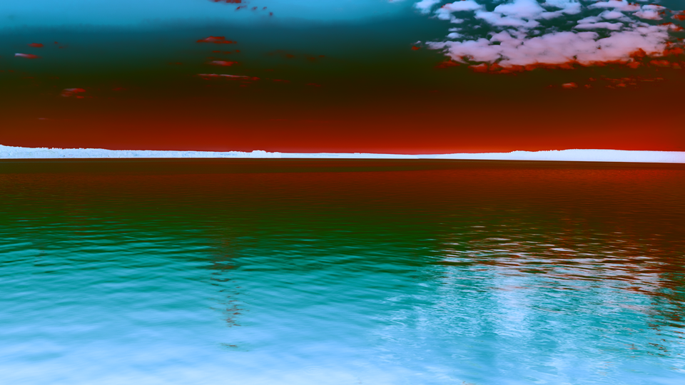
 Equidensity Contour Map — simulated result across source images.
Exercise Illustration
A description of the exercise illustration.
Learning Outcomes
Combine equidensity mode with W-Curve and metallic tinting for a scientific-visualization-style contour map.
Key Concepts
- Equidensity doubles the solarization dip, creating sharp tonal bands
- W-Curve adds additional fold points, multiplying the bands
- Metallic tinting colors the result based on brightness
Video Source
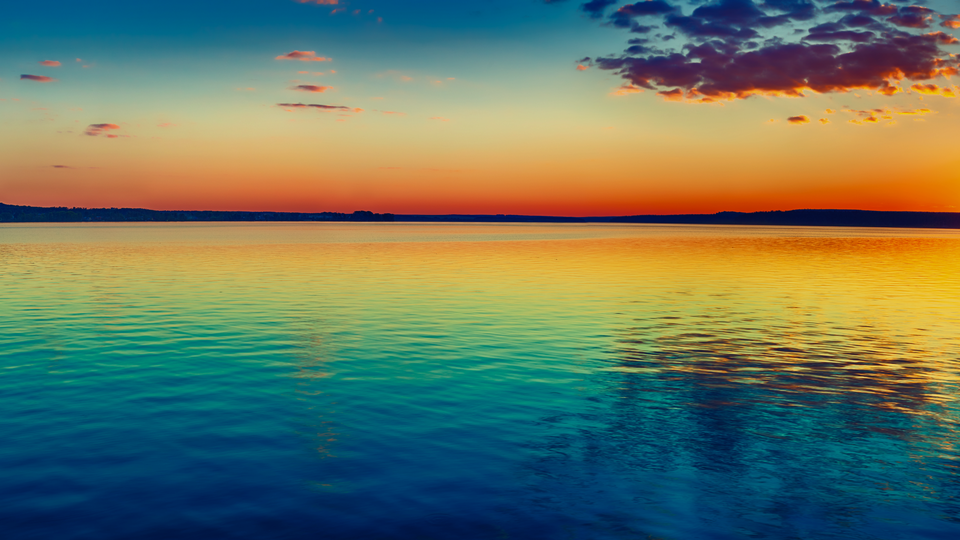
Footage with broad, gradual tonal transitions (a sunset, studio lighting, or slow-moving clouds.)
Steps
- Enable equidensity: Toggle Equidensity (Switch 7) to On and set Y Inversion (Knob 1) to about 80%. The image divides into discrete luminance zones separated by dark contour lines.
- Switch to W-Curve: Toggle Curve Shape (Switch 10) to W-Curve. Additional contour bands appear as the two-peaked proximity function creates more fold boundaries.
- Add chroma processing: Set Channel (Switch 9) to YUV and increase UV Inversion (Knob 2) to about 60%. The color channels also divide into zones.
- Add Mackie lines: Increase Mackie Gain (Knob 3) to about 60% and set Threshold (Knob 6) to about 50%. Bright lines trace the contour boundaries.
- Metallic finish: Toggle Metallic (Switch 11) to On. The entire image is tinted with a strong blue-cyan metallic sheen, with brighter contour areas receiving the strongest color shift.
- Adjust mix: Sweep Mix (Fader 12) to blend the contour map with the original footage.
Settings
| Control | Value |
|---|---|
| Y Inversion | 80% |
| UV Inversion | 60% |
| Mackie Gain | 60% |
| Mackie Width | 30% |
| Tint | 50% |
| Threshold | 50% |
| Equidensity | On |
| Polarity | Positive |
| Channel | YUV |
| Curve Shape | W-Curve |
| Metallic | On |
| Mix | 100% |
Glossary
-
Equidensity: A photographic technique using specialized film to render constant-density (iso-luminance) regions as discrete bands, used in scientific imaging.
-
Gradient Detection: Measuring the rate of change between adjacent pixel values to identify edges or tonal boundaries.
-
IIR Filter: Infinite impulse response filter; a digital filter whose output depends on both current input and previous output, creating exponential decay and temporal smoothing.
-
Mackie Line: A bright contour artifact at tonal boundaries in solarized images, caused by lateral bromide migration during darkroom development.
-
Midtone: The range of tonal values between deep shadows and bright highlights; in a 10-bit signal, values near 512.
-
Polarity: The orientation of tonal values; positive polarity preserves the original mapping, negative polarity complements it (1023 − value).
-
Proximity Function: A piecewise function measuring distance from a midtone center; Sabattier uses triangle (S-curve) and dual-triangle (W-curve) variants.
-
Pseudo-Solarization: Partial tonal reversal caused by re-exposing a photographic print during development, distinct from true solarization.
-
Tonal Fold: The visual effect of subtracting a midtone-peaked curve from the signal, causing a portion of the tonal range to reverse direction.